|
|
Link to slides used for this paper as presented at the conference. They are in Acrobat PDF format.
|
|
![]()
John Clyne and John Dennis
National Center for Atmospheric Research
Scientific Computing Division
Direct Volume Rendering (DVR) is a powerful volume visualization technique for exploring complex three and four-dimensional scalar data sets. Unlike traditional surface-fitting approaches, which map volume data into geometric primitives and can thus benefit greatly from widely available commercial graphics hardware, computationally-expensive DVR is performed, with rare exception exclusively on the CPU. Fortunately DVR algorithms tend to parallelize readily and much prior work has been done to produce parallel volume renderers capable of visualizing static datasets in real-time. Our contribution to the field is a shared-memory implementation of a parallel rendering package that takes advantage of high-bandwidth networking and storage to deliver volume rendering of time-varying datasets at interactive rates. We discuss our experiences with the system on the SGI Origin2000 supercomputer.
In recent years, Direct Volume Rendering (DVR) has proven to be a powerful tool for the analysis of time-varying, three-dimensional scalar datasets associated with the atmospheric, oceanic and astrophysical sciences. The benefits of DVR, probabilistic data classification [4], and direct projection of volume samples are key to producing insightful visualizations of simulation results, rich with amorphous and fluid-like features [3]. Animations of spatial rotations at a single instance of time can clarify three-dimensional structure, while temporal animations can show the evolution of three-dimensional structure and depict complex dynamics.
Visual data exploration is an inherently interactive process. To fully exploit the power of DVR as an analysis tool, interactive frame rates (at least 5Hz) must be achieved. Static images or animations produced through a batch process that represent complex 3D phenomena may be of limited value. Invariably, features of interest are obscured, improperly classified, or poorly lit. Unlike more conventional visualization techniques, which map data into geometric primitives that can then be efficiently displayed using hardware graphics accelerators, DVR algorithms generally do not benefit from commercially available hardware: the computationally expensive process must be carried out entirely on the CPU.
Fortunately, DVR algorithms tend to parallelize nicely, and much work has been done in the area of accelerating DVR methods for static data [5,7,14,8,12,1,9,13]. Interactive volume rendering of single time-steps is now within the reach of many researchers. However, temporal animations must still be produced through a batch process. Researchers can use interactive tools to determine classification functions, color mappings, and to select view points, but the production of the temporal animation must then be carried out as a batch process and subsequently viewed as a pre-recorded animation. If initial viewing parameters selected from representative time-steps are not correct for the entire time-series, the painstaking, error-prone process must be repeated.
Time-varying datasets impose additional costs that have made interactive rendering difficult to achieve. The principal culprit is I/O. Rendering a moderately sized (2563) dataset made up of 8-bit voxels at a frame rate of 10 Hz would require an input pipe capable of delivering a sustained bandwidth of over 150 MBytes/sec. Though improvements in online magnetic storage technology have not kept pace with processor technology advances, the availability of both software and hardware-based RAID systems, which exploit parallelism by using arrays of disk drives, has provided a practical means to achieve sustained I/O transfer rates in excess of 100 MBytes/second [11].
In [2], we describe a volume-rendering system based on a parallel implementation of Lacroute's Shear-Warp Factorization algorithm [6], that is capable of rendering and displaying to the desktop, time-varying 2562 X 175datasets at 4 Hz on a 16-processor, Distributed Shared Memory (DSM), HP Exemplar SPP2000. Our volume rendering system, "Volsh," achieves this result by taking advantage of commercially available multiprocessors and high-bandwidth networking and storage. In this paper we describe our preliminary experiences with Volsh on another DSM: an SGI Origin2000.
The remainder of this paper is organized in four sections: Section 2 briefly discusses the rendering algorithm and our parallelization strategy. A detailed description appears in [2]. Section 3 we presents an overview of the rendering system and discusses its implementation. Section 4 presents performance results for Volsh running on an SGI Origin2000. Section 5 discusses these results and suggests areas for future work.
The Volsh volume rendering system is based on a parallel implementation of the Shear-Warp Factorization algorithm. The serial version of this algorithm is among the fastest reported in the research literature. There have been a number of successful parallel implementations, spanning a variety of different computer architectures [5,12,1]. Parallel implementations are capable of rendering moderately sized (2563) static datasets at interactive rates. We extend an existing serial implementation of the Shear-Warp Factorization algorithm [5], parallelizing the code and optimizing its support of time-varying data.
The Shear-Warp algorithm operates by applying an affine viewing transformation to transform object space into an intermediate coordinate system called sheared object space. Sheared object space is defined by construction such that all viewing rays are parallel to the third coordinate axis and perpendicular to the volume slices. Volumes are assumed to be sampled on a rectilinear grid. For a parallel projection, the viewing transformation is simply a series of translations. Note that because all voxels are translated by the same amount within a given slice, the resampling weights are invariant within each slice. After the slices have been translated and resampled, they may be efficiently composited in front-to-back order using the over operator to produce an intermediate, warped image. The distorted, intermediate image must then be resampled into final image space.
The Shear-Warp algorithm can operate directly on raw data, or the data may first be classified in a pre-processing step. The pre-processing step calculates voxel normals and opacities and uses run-length encoding (RLE) to record contiguous runs of transparent voxels. The advantages of using RLE data are twofold: 1) The renderer can exploit coherency in the dataset, quickly skipping over transparent voxels. 2) Expensive calculations, such as computing the voxel normals, are performed offline, reducing the amount of work the renderer is required to perform. The disadvantages to rendering RLE data are: 1) The classification function is fixed and cannot be modified during rendering. 2) The storage requirements for the RLE data may be substantially larger than the original, scalar data.
Execution time for the RLE algorithm is dominated by three calculations: 1) Projection of the volume into the intermediate image. 2) Warping the intermediate image into the final image. 3) Computing the view-dependent portion of a lookup table used for shading. The raw data algorithm must perform the additional step of computing gradient vectors and determining voxel opacity values. We parallelize each of these computational phases and synchronize all processors between each computational phase.
Projection of the 3D volume, which involves resampling and compositing the volume slices, is by far the most computationally expensive task in the RLE algorithm and also the most challenging to efficiently implement in parallel. To minimize processor synchronization, we partition tasks based on an image-space decomposition of the intermediate image. Each processor is responsible for computing a number of scanlines in the intermediate (warped) image. The image is partitioned into small groups of contiguous scanlines. Initially processors are statically assigned groups of scanlines in cyclical fashion. As the calculation proceeds, dynamic task stealing is used to perform load balancing [9]. Each processor maintains its own queue of groups of scanlines. As soon as a processor finishes all its groups, it tries to steal a group of scanlines from its neighbors. This process continues until the projection is complete. Our task-stealing algorithm differs from Levoy's in that processors only look to a limited number of neighbors for additional work.
Parallelizing the 8k-entry shading lookup table, typically accounting for 10% of the total calculation time in the RLE algorithm, is trivial and results in an embarrassingly parallel computation. There are no interdependencies between table entries; we simply divide the table entry computations equally among the processors.
Resampling the intermediate image is the least expensive of these tasks, typically representing 5% of the total calculation for the RLE renderer. We partition the workload by dividing the final image into P groups of adjacent scanlines, where P is the number of processors, and statically assign one group of scanlines to each processor. There are no pixel interdependencies in the final image, thus no synchronization is required.
The raw data algorithm requires the additional step of classifying the data and computing normal vectors. Classification is specified via a user-defined lookup table. Normalized normal vectors, which are estimated using the central differences method and encoded as 13-bit integers, are calculated using lookup tables to avoid expensive division and square root operations. We easily parallelize the classification step by partitioning the volume into contiguous, axis-aligned slabs and assigning each processor a single slab.
Time-varying data incur additional execution costs primarily due to I/O. The techniques we employ to help address these costs are to utilize high-bandwidth, striped disk arrays and to pipeline the rendering and reading tasks, "hiding" the I/O behind the rendering calculations. We spawn separate I/O and rendering threads, double-buffering reads of the data volume files. We use a parallel memory copy to move the input data from the read buffer into the application buffer. If I/O time is less than rendering time, we can mask the cost of I/O and theoretically achieve rendering rates comparable to that for static data. If the I/O time is greater than that of the rendering calculation, then we are I/O bound and limited by the rate at which we can read and distribute data.
There are tradeoffs to be considered between the RLE and raw data rendering algorithms when addressing time-varying data. The RLE algorithm is typically faster than the raw data algorithm because it exploits data coherency. However, the RLE data volumes may be substantially larger than the original raw data volumes and have correspondingly greater I/O requirements. The RLE data volumes contain additional information (gradient and opacity) and three view-dependent copies of the volume need to be maintained. The exact size of the RLE volume is largely determined by the user-defined classification function: the more voxels that are mapped to zero opacity, the smaller the RLE volume.
The Volsh rendering system supports two user interfaces. The first is a batch utility, driven by a Tcl script. The Tcl interface facilitates batching complex rendering tasks and gathering performance measurements. A list of rendering instructions and data volumes are ingested, and a stream of RGB images is output to a file.
The second user interface is an interactive application with an X11-based graphical user interface (GUI). Large multiprocessor systems typically do not have directly attached display devices. To address this issue, the interactive system is implemented as two separate UNIX processes that communicate via sockets. One process runs on the parallel machine, performing rendering and managing the GUI. The second process runs on a display host and is responsible for posting the 24-bit RGB imagery, transmitted from the renderer, to the frame buffer via the OpenGL API.
The original serial-rendering algorithm and the extensions we've added are implemented in the C language. The user interfaces are implemented in C and C++. Parallelization is accomplished using POSIX threads (pthreads), making the software portable to most shared-memory architectures.
Voxels in the raw datasets are 8-bit quantities. RLE voxels are 32 bits: the original sample value is represented by 8 bits and the remaining 24 bits are used to represent gradient magnitude (8 bits) and an encoded representation of a gradient (13 bits).
The results reported in the performance section were collected on a 64-node, 128-processor SGI Origin2000. We report results obtained using 1 to 16 processors. Each processor is a 250 MHz R10000 CPU with 4 MBytes of cache. Each node board has 256 MBytes of memory. The disk subsystem is a level 0 RAID, implemented with IRIX software striping, consisting of 28 drives striped across 5 Fibre Channel controllers, using a stripe unit of 65 Kbytes per drive. Each disk is a 9 GB Seagate drive with a 7200 rpm rotation rate. The maximum sustained bandwidth that we have measured for read operations on the disk array using direct I/O and 4 MByte reads is 300 MBytes per second. For indirect I/O, the maximum sustained rate we've measured is 90MB's per second. Our volume rendering system is currently implemented using indirect I/O. Performance measurements on the disk array were made with the xdd utility [11]. The Origin is networked to a display host, an Onyx2/IR, via switched 100 Mbit Ethernet.
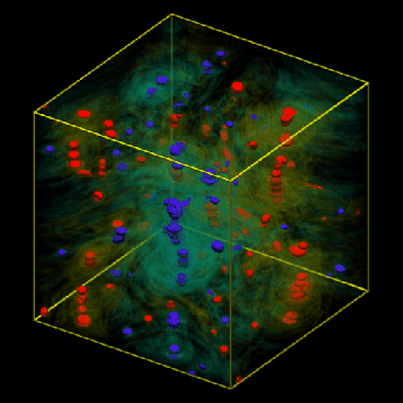
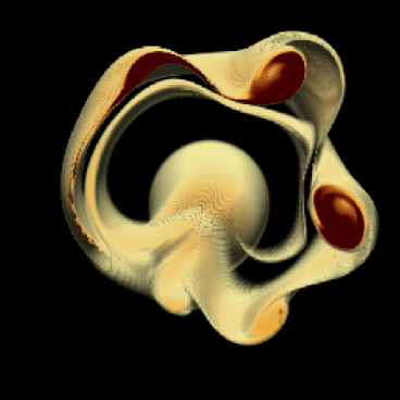
We use two different datasets to evaluate the performance of the rendering system. The Quasi-Geostrophic (QG) data (see Figure 1) are computer simulation results depicting the formation of coherent structures in rotating, incompressible, turbulent fluid flow. These data and the classification functions chosen for them are of particular interest to us in exploring performance characteristics because they are dense and rich with amorphous features; their computational needs, and in the case of the RLE version, their I/O needs are extremely demanding. The second dataset was produced from a simulation of the wintertime stratospheric polar vortex [10]. The polar vortex (PV) data (see Figure 2) are relatively sparse and opaque, exhibiting a great deal of coherence throughout the entire simulation; their computational and I/O needs are much more easily satisfied.
|
|
|
|
Table 1 lists the datasets, their spatial resolution, the size of each raw time-step, and the average size of each RLE time-step. In Table 1, note that the relative sizes of a raw and corresponding RLE dataset provide a measure of spatial coherency. The larger the RLE dataset relative to the raw dataset, the less coherency exists. The RLE version of the QG dataset is over five times as large as the raw version. However, the RLE version of the PV dataset is not much larger than the raw version. Note also that the spatial resolution of the PV volumes is over four times that of the QG volumes.
|
|
In the experiments reported below, all data are read directly from disk. Individual volume files are concatenated into larger, multi-volume files to improve I/O performance. The kernel buffer cache was flushed prior to running each experiment. Unless otherwise specified, all results are for single-light, Phong-illuminated, monoscopic, three-channel (RGB), 256x256 resolution imagery. Each experiment renders 100 time-steps from a fixed viewpoint.
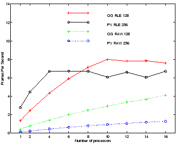
Figure 3 plots frame rates vs. number of processors for rendering raw and RLE versions of the QG and PV datasets. We see from Figure 3 that, with the exception of the raw version of the PV dataset, all of the datasets can be rendered at interactive rates. We also observe that both RLE datasets reach a peak frame rate on relatively few processors, and then performance goes flat and even declines for some processor runs. Contrarily, the performance curves for the raw data, while never achieving the same frame rate as the RLE data, steadily increase from 1 to 16. We examine both of these phenomena more closely below. Last, we note that despite the much greater spatial resolution of the PV data, the rendering times for it are comparable to that of the lower resolution QG data, particularly in the case of the RLE versions of the datasets. This result reflects the greater coherency found within the PV data.
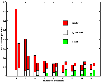
Figure 4 plots execution time of the major components of the rendering system for RLE data vs. number of processors. The render parameter includes projection, shade-table calculation, and the 2D image warp. The i_overhead parameter depicts the overhead costs of performing double-buffered input. These overheads essentially reflect the cost of copying data from the double-buffer into the application space using a parallel memory copy. We note that the parallel memory copy does not scale beyond four processors. We discuss this issue in the next section. The last parameter, i_wait, depicts the unmaskable, double-buffered I/O time for reading data. When the task is computationally (render) bound, i_wait is close to zero. As the rendering process is sped up through the addition of more processors, the task can become I/O bound, and i_wait will grow. Growth in the i_wait parameter corresponds to the points in Figure 3 where performance goes flat for the RLE versions of the datasets.
|
|
|
|
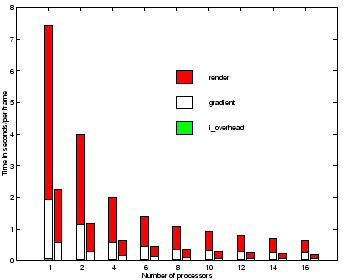
Figure 5 plots execution time of the major components of the rendering system for raw data vs. number of processors. The render and i_overhead parameters represent the same information as in Figure 4. There is no corresponding i_wait parameter in Figure 5 because the input wait time is zero for all of the processor runs; the raw datasets, because of their smaller size and increased rendering costs, are completely computationally bound. The gradient parameter depicts the execution time to compute normal gradients required by the raw datasets. We observe that the gradient calculation represents a significant portion of the total display time, taking anywhere from 1/3 to 1/2 of the render time. We also observe that gradient calculation scales poorly. The PV data achieves an efficiency of only 50% on 16 processors, while the rendering calculation achieves an efficiency of 90%.
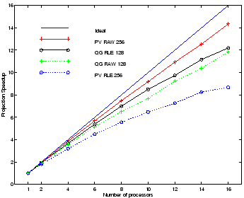
Figure 6 shows speedup for the projection calculation, the most expensive component of the rendering algorithm, for all four datasets. We observe that the speedup varies widely. The raw version of the QG dataset demonstrates the best efficiency, while the RLE version of this same dataset demonstrates the worst efficiency. Both the raw and RLE versions of the QG data perform comparably well.
|
|
|
|
We have demonstrated that Volsh is capable of delivering interactive rendering rates for time-varying data using, in some cases, relatively few processors on the Origin2000 class of supercomputers. While interactive rendering is possible, the multiprocessor speedup associated with various components of the rendering system - the gradient, projection calculation, and parallel memory copy - is not ideal. We conclude this paper with some discussion about why these components are not exhibiting better performance. As this paper goes to press, we note that NCAR's Origin system will have been on the machine room floor for only a matter of weeks. The opportunity to perform a rigorous analysis of these problems is not available to us and we can only offer our speculations at this time.
We believe that all of the performance problems we've witnessed and discussed are related to a single issue: memory layout. The parallel implementation of Volsh targets a generic shared-memory system. No architecture-specific assumptions have been made. Early indications suggest that the Origin's DSM architecture demands greater consideration with regard to memory placement to achieve optimal performance. Our simplisitic initial approach results in having all memory allocated to a single node board. As the number of processors used by the application is increased, the contention for that single node board becomes significant. This contention is particularly evident by the poor scaling of the parallel memory copy which performs no calculation and whose performance is completely characterized by memory access speeds.
Memory allocation problems may be futher compounded by our choice of pthreads for our parallelization construct. The pthread interface provides no facilities for specifying any affinity between a process and memory. There is no way to ensure that a thread is run on any particular processor and therefore no way to ensure that it accesses only local memory. Consequently, we may not be able to obtain optimal results without selecting another parallelization construct, for example, the SGI's sproc interface or C language programming extensions. To test this theory, we have implemented a parallel memory copy using SGI's C language extensions. These extensions permit explicit memory placement, and using them we have witnessed near-linear speedup. Unfortunately, in IRIX 6.5SE, pthreads and C language parallelization constructs cannot be intermixed.
Improving speedup of the computational components of the rendering system would improve rendering performance of the raw data, but would not improve the performance of the RLE datasets. These data quickly become I/O bound while rendering performance continues to scale, albeit poorly. For portability and ease of implementation, we elected to use indirect I/O, limiting read bandwidth to 90 MBytes per second. A direct I/O implementation could conceivably ingest data at 300 MBytes per second on our Origin configuration, permitting higher frame rates, possibly suitable for VR purposes, or permiting the exploration of even larger datasets.
We would like to acknowledge the National Center for Atmospheric Research, which is operated by the University Corporation for Atmospheric Research under the sponsorship of the National Science Foundation. We also acknowledge Dr. Jeff Weiss for providing us with the QG dataset, Dr. Mark Taylor for the Polar Vortex dataset, Jeff Boote for his assistance with the GUI, and the entire SCD Supercoming Systems Group for their assistance with benchmarking.
![]()