
Stephen Bique
stephen.bique@nrl.navy.mil, robert.rosenberg@nrl.navy.mil
Presented at Cray User Group 2009 Conference, May 4-7, 2009
| xn+1 = (αxn + c) mod m, n ≥ 0, | (1) |
A special case of the LCG is a multiplicative congruential generator (MCG) with “increment” c =0:
| xn+1 = α⋅xn mod m | (2) |
Avoid choosing a small modulus m whenever a large number of random numbers are needed (because the period is always bounded by m). The largest period possible for an MCG can be achieved provided the multiplier is a “primitive root” whenever the modulus is a prime number because Euler's φ(m), the number of integers between 1 and m and relatively prime to m, is exactly the m − 1 integers less than m. This fact from elementary number theory is next briefly explained. Given an integer m , the “order” of any integer α is the smallest integer n such that
| αn mod m = 1. | (3) |
| α(m−1) ⁄ f mod m ≠ 1 | (4) |
| (α ⊗ β) mod m = ( ( α mod m) ⊗ (β mod m) ) mod m | (5) |
| p = q⋅n + r, 0 ≤ r < n. | (6) |
| 1 = αp mod m by supposition | |
| = α q ⋅ n + r mod m by (6) | |
| = ( α q ⋅ n⋅ αr ) mod m | |
| = αr mod m by (5) | (7) |
| Σψ(f) = m−1 = Σφ(f). | (8) |
| 1 | , | 2 | , | 3 | , | …, | n−1 | , | n | , |
n |
n |
n |
n |
n |
||||||
Usually it is easy to find small primitive roots regardless of the magnitude of the prime modulus. So it is practical to search for a primitive root starting from small primes. For example, using both the GNU Multiple Precision (MP) “Bignum” arithmetic (GMP) and the NTL libraries (with GMP) [6][7], we found that 11 is a primitive root of the prime 48047305725 ⋅ 2172404 − 1 = 286445162615702949817…(16 pages worth of digits omitted)… 30342041599, which has exactly 51, 910 decimal digits (we counted using the UNIX command wc). This number is prime because 48047305725 ⋅ 2172403−1 (which we confirm has the same number of digits base 10) is currently the largest known Sophie Germain prime (with high probability), which is any prime number p for which 2p+1 is also prime [8]. Such primes simplify the task of finding primitive roots. To show that a small number α is a primitive root of a large prime 2p+1 where p is prime, it is only necessary to verify αp ≠ 1. The reason is there are only two exponents that need to be checked by equation (4), namely 2p ⁄ p = 2 and 2p ⁄ 2 = p. Plainly α2 mod (2p+1) ≠ 1 since for small primes α, α2 << 2p+1.
Is there a sound approach to find constants for an MCG in a parallel setting using Sophie Germain primes? Search for a primitive root r of a prime modulus m = 2p+1, where p is a Sophie Germain prime, and then employ rt as the multiplier for some suitable power t of the primitive root r [9]. Technically it is incorrect to say “Sophie-Germain primes as the prime modulus” [9] because p is the Sophie Germain prime, not m = 2p+1. For example, in [9] it is erroneously stated that m = 264 − 21017 is a Sophie Germain prime (2m + 1 = 265 − 42033 = 36893488147419061199 = 23 ⋅ 383 ⋅ 42013 ⋅ 253637 ⋅ 393031 is evidently not prime), although p = 9223372036854765299 is a Sophie Germain prime with 2p + 1 = 264 − 21017. Mersenne primes provide slightly better performance compared to using Sophie Germain primes but there are far fewer of them [9][10]. While there is a sound basis for using primes near a power of two as the modulus, the case for using Sophie Germain primes in not compelling.
A primitive root is discovered fairly quickly. Yet a small primitive root is unlikely a good multiplier for an MCG using a large modulus m. Is r n mod m a primitive root whenever r is a primitive root of a prime number? The powers of r (mod m) generate all of the integers 1, 2, …, m − 1, and they cannot all be primitive roots because some exponents must divide m−1, which is even. All of the primitive roots belong to the set| { r n | gcd(m−1,n) = 1 }. | (9) |
Thus the number of primitive roots is the number of positive integers less than the prime modulus m that are not multiples of factors of m−1, which was discovered in the 19th century by Keferstein [3]. Regardless of the choice of the prime modulus and corresponding primitive root as a multiplier, terms of an MCG sequence with shift half of the period are highly correlated [11]. This fact favors employing large moduli m so that half the period (m−1) ⁄ 2 is sufficiently large.
Factoring large integers using trial and error is practical only about 90% of the time. The reason is that given any sequence of 100 integers, most of them are divisible by 2 (50%), 3 (33%), 5 (20%), and other small primes. Hence, not all integers are equally easy to factor. The SQUare FOrms Factorization algorithm can factor almost any integer with up to 18 digits [12][13]. Yet the algorithm may be useful when the word size is 128-bit or larger. Unlike the vast majority of factoring algorithms, the SQUFOF algorithm works best using mainly integer arithmetic.
We developed a fast variation of the SQUFOF algorithm. Our implementation in C is successful around 97% of the time for large integers up to 264 (higher success rate is possible with reduced performance). While finding a factor may not be a trivial task for large integers, determining if any given integer has a non-trivial factor (i.e., is composite) can be decided quickly with high probability using the Rabin-Miller Probabilistic Algorithm, which was invented in the mid-1970's [14]. When the algorithm is correctly implemented, a program that asserts an integer is composite cannot be wrong. Perhaps a single composite among about 1020 integers will be indistinguishable from a prime number using the Rabin-Miller Probabilistic Algorithm.
Even when the number of factors is small and can be discovered reasonably fast, raising an integer to a large power via modular arithmetic is accomplished quickly and precisely but cannot be done using typical library functions. Identity (5) is useful to perform such computations. This identity is not typically covered extensively in computer science curricula. We developed a fast implementation in C to do such computations on unsigned integers. An implementation in C to perform modular multiplication on signed integers is published [15].
The popularity of MCGs has spawned an abundance of research in both sequential and parallel settings. Recently, a new approach to find optimal multipliers was proposed based on the “figures of merit”, a measure that was introduced in 1976 [16][17]. Generally it is impractical to conduct an exhaustive search to find optimal parameters suitable for sequential computations. In a parallel setting, there is no evidence to suggest that there exists any method of pseudorandom number generation that would be ideal for all applications. Regardless, packages for scalable pseudorandom number generation do exist [18].
Although a large body of knowledge exists on choosing parameters for an MCG, the theory is incomplete. For example, a statement such as “The multiplier is chosen to be certain powers of 13 … that give maximal period sequences of acceptable quality” [9] is sound, yet does not prescribe an algorithm. A programmer developing an application would find a table of parameters for an MCG useful. Yet, it is not easy to find a single multiplier for an MCG in many published works (see for example [9] or [10]). Moreover, practical issues are often inadequately addressed. For example, the period may be considerably smaller than theoretically possible due to computer arithmetic so that the effective period is p½, where p denotes the theoretical period [19].
Our primary interest is to compute pseudorandom numbers in parallel while avoiding the computation of any subsequence produced by another process. Whenever two processes produce the same subsequence, we say that “overlap” has occurred. A natural idea is to use a different seed but to be certain that overlap is avoided, it is advisable to implement some “leapfrog” technique to partition the sequence among the processes, which may be appropriate if scalability is not a concern [20]. Although the leapfrog method is sound, we prefer a simpler approach that does not require additional computations whenever the number of processes is changed.
We seek a simple, fast implementation of an MCG which not only produces good results in a parallel setting for many applications, but also is easily adapted to run on different sets of processors, i.e., scalable in the sense that performance and quality remain high while the effort required to modify the code is minimal. In the next section, we focus on performance. Subsequently we prescribe ways to find prime moduli and good multipliers for an MCG. We present data based on our algorithms and then conduct some experiments to assess the quality of the results.
When the modulus is a power of two, there is a computational advantage in performing the modulus operation for an MCG (using a fast bit-wise and operation). There is also a performance benefit when the modulus is a Mersenne or Sophie Germain prime [9][10]. Actually this advantage holds more generally for any prime sufficiently close to a power of two, which we demonstrate next.
For an MCG (2), fix m = 2q − k for arbitrary positive integers q > 1, k ≥ 1. Write
| α⋅xn = γ 2q + λ, | (10) |
| γ 2q + λ = γ 2q + (kγ − kγ) + λ = γ (2q − k) + kγ + λ. | (11) |
| xn+1 = α⋅xn mod m = (kγ + λ) mod m. | (12) |
Example
Choose the prime modulus m = 13 with q = 4 and k = 3. Take α = 11 which is a primitive root of 13. Set x0 = 12, which is a valid seed for an MCG. Then αx0 = 11⋅12 = 132 = 8 ⋅ 24 + 4, which yields γ = 8 and λ = 4. Hence, k γ + λ = 3 ⋅ 8 + 4 = 28 > 26 = 2m.
How large can γ be? For sufficiently small k, we claim
| γ < 2q − 2(k+1) . | (13) |
| α⋅xn < (m − 1)2 = (2q − k − 1)2 = 22q − 2q+1(k+1) + (k+1)2. | (14) |
We know every nonnegative integer can be expressed as 2q − k for some integers q and k. In particular, for every prime integer m with 2 < m < 2q, if m is sufficiently close to 2q, then there exists a small integer k such that m = 2q − k. We shall only consider integers k satisfying
| 1 ≤ k < 2(q−1)/2. | (15) |
| (k+1)2 ≤ ( 2(q−1)/2 )2 ≤ 2q−1 < 2q. | (16) |
In view of this inequality (16), upon dividing both sides of the inequality (14) by 2q, we see that the claim (13) holds:
| γ = | α⋅xn | < | 22q − 2q+1(k+1) + (k+1)2 | = 2q − 2(k+1) . |
2q |
2q |
In the case of a Mersenne prime m = 2q − 1, we need perform at most a single subtraction operation to perform the mod m operation in equation (12). Indeed, k = 1 and in view of the claim (13), we must have that
| kγ + λ − m = γ + λ − m < 2q − 4 + 2q − 1 − m = 2q+1 − 5 − m = 2q+1 − 5 − (2q − 1) = 2q − 4 < m. | (17) |
Example
Consider the miniscule Mersenne prime modulus m = 7 for illustration purposes. Choose the primitive root α = 5. Set the seed x0 = 5. Then &gamma = 5⋅5 ⁄ 8 = 3 < 2q- 2(1+1) = 4. This shows the upper bound predicted by (13) is tight. The sequence generated by the MCG (2) is 5,4,6,2,3,1, …, is calculated using γ + &lambda [ − m if needed] as follows: 3 + 1 = 4, 2 + 4 = 6, 3 + 6 − 7 = 2, 1 + 2 = 3, 1 + 7 − 7 = 1. Observe one third of the time subtraction is needed and the largest γ+λ−m value is 2 (compute x3 given x2 = 6) and this maximum value is smaller than 23 − 4 = 4 as the inequality (17) asserts.
Algorithm 1: MCG Computation for Mersenne Primes
Recall, we may have that kγ + λ > 2m. How large can kγ + λ be if m is not a Mersenne prime? Consider a recursive application of equation (12) replacing α⋅xn by kγ + λ to obtain new upper γ’ and lower λ’ “q-bits.” We compute
| kγ’ + λ’ = k ⋅ | kγ + λ | + λ’ ≤ k ⋅ | k(2q − 2(k+1) −1) + (2q−1) | + λ’ | ||
2q |
2q |
|||||
| = k ⋅ | 2q(k+1) −2k(k+1) − (k+1) | + λ’ ≤ k(k+1) +λ’ ≤ 2q−1 + 2q − 1 = 3⋅2q−1 − 1, | |||
2q |
|||||
| kγ’ + λ’ − m < 3⋅2q−1 − 1 − (2q − k) = 2q − 1 + k − 1 < m, | (19) |
Example
Consider the prime modulus m = 1021 which is neither a Mersenne prime (because the distance to the nearest power of two exceeds one) nor a Sophie Germain prime (because 2m+1 = 2043 is not prime). Write m = 210 − 3, i.e., q = 10 and k = 3. Notice inequality (15) is satisfied because (10 − 1) ⁄ 2 = 4 > k > 1. Choose the multiplier α = 991, which is the largest primitive root of 1021. Employ the seed x0 = 987. Using these choices, the MCG (2) has period 1021. To calculate x1 we find kγ + λ = 3⋅955 + 197 = 3062 and in the recursive step we find the next pseudorandom number is 6 + 1014 = 1020. The largest γ computed in the first step is 987 < 210 − 8 as predicted by (13). Subtraction is needed only twice when the previous pseudorandom number is 68 and 34. In this case, subtraction is never needed when the recursive step is performed. The recursive step is needed nearly 83% of the time.
Example
Consider the prime modulus m = 1048573. Note m = 220 − 3, i.e., q = 20 and k = 3. Choose the multiplier α = 2, which is a primitive root of 1048573. Take the seed x0 = 1048572. Using these choices, the MCG (2) has full period 1048572. Subtraction is needed only once and the recursive step is never performed! Unfortunately the sequence does not appear random since every number is twice the previous number mod m. This example demonstrates that merely having an optimal period does not provide any assurance on the quality of the sequence.
Consider changing only the multiplier in the previous example, setting α = 828119 which is a primitive root of 1048573. Using these choices, the MCG (2) has full period 1048572. Subtraction is needed a total of four out of 1,048,572 times, including twice after performing the recursive step (after generating the numbers 854996 and 641247). The recursive step is needed nearly 79% of the time.
Example
The CRAY RANF is a MCG given by xn = 44485709377909⋅xn − 1 mod 281474976710656, which has period 246 [21]. This period seems to be valid (more on this later) using direct calculation with the usual operators (* and %) in C, i.e., perform the modulo operation in (2).
Example
Consider the prime modulus m = 281474976597361 = 248 − 113295. Choose the multiplier α = 582167988922 and the seed x0 = 281474976597360. Then implementing the previous algorithm in C yields the period 18936324 ≈ (248)½. Performing the computations exactly (and more slowly), the period should be 281474976597360 = 248 − 113296. Using an efficient implementation based on the GMP library on the CRAY XD1, merely computing (without saving or printing) the full sequence would take about 268 days (ignoring crashes!).
| LCG | Implementation in C | χ2 | Time (s) |
|---|---|---|---|
| 1327760490⋅xn mod 231−1 | Algorithm 1 | 1.19 | 11.0 |
| 97693434⋅xn mod 237−25 | Algorithm 2 | 0.926 | 14.1 |
| 27355192⋅xn mod 238−45 | Algorithm 2 | 6.36 | 14.0 |
| 247016489220937⋅xn mod 248−59 | Algorithm 2 | 78.0 | 13.2 |
| 14022294538115072⋅xn mod 255−55 | Algorithm 2 | 6.74 | 13.2 |
| 10337092905140992⋅xn mod 256−5 | Algorithm 2 | 5.69 | 13.2 |
| 98530843867429240⋅xn mod 257−13 | Algorithm 2 | 4.95 | 13.2 |
| 72103240369675328⋅xn mod 258−27 | Algorithm 2 | 4.53 | 13.2 |
| 2209592322954132280⋅xn mod 261−1 | Algorithm 1 | 3.91 | 11.0 |
| 5048131329874245129⋅xn mod 263−25 | Algorithm 2 | 2.05 | 13.2 |
| RANF: 44485709377909⋅xn mod 248 | 44485709377909*xn % m | 1610612748 | 58.9 |
| 25214903917⋅xn + 11 mod 248 | lrand48() | 4.35 | 32.4 |
| 25214903917⋅xn + 11 mod 248 | drand48() | 2.70 | 50.9 |
The die is determined using modular arithmetic, e.g., lrand48() % 6 + 1, except in the implementation that uses drand48() for which the side is 6*drand48() + 1. The chi-square χ2 statistic is computed assuming a uniform distribution (we expect to roll each side of the die approximately 228 times.) The CRAY RANF function only rolls three of the six possible outcomes (which three sides depends on the seed)! Note we are using usual C operators (not calling the FORTRAN routine) so that we can compare the cost savings by not performing the modulo operation. Both Algorithms 1 and 2 are implemented in a straightforward manner. Except for the RAND48 library calls, we seed the generator using m − 1, where m is the modulus. We initialize drand48() and lrand48() by calling seed48(A), where A denotes the array of shorts [0x1234, 0xabcd, 0x330e].
A fast implementation of Algorithm 1 or 2 is easily coded. The number γ is obtained by shifting q bits to the right. The integer λ is calculated by performing a bit-wise and operation with 2q − 1. When q = 64, do not apply the algorithm since γ is zero and instead use direct calculation (2). As the modulo operation is relatively slow as we have shown, we recommend using moduli < 263.
Example
Consider the prime modulus m = 18446744073709549363 = 264 − 2253. Choose the multiplier α = 1262014585074097263 and the seed x0 = m − 1. Then implementing Algorithm 2 in C produces xn = 0 for all n ≥ 63. If we abandon Algorithm 2 and perform the computations in C directly (as xn = α * xn − 1 % m), the period is long.
We see that performing the modulo operation is relatively slow. Our algorithms are fast compared to calling library functions. Using Mersenne primes (Algorithm 1), we see the speedup is about 1.2× compared to an implementation of Algorithm 2. We have settled important implementation issues to achieve a fast implementation of an MCG. We next address how to find constants to use in an MCG so that the generated sequence is high-quality.
The main requirement is that the modulus m = 2q − k, is a prime close to a power of two satisfying inequality (15). Consider a few different strategies to select such prime modulus:
Recall, it has been argued that using Sophie Germain primes as prime moduli makes it easy to find primitive roots [9]. However, it is not the prime modulus m which should be a Sophie Germain prime, but rather (m − 1) ⁄ 2 which should be a Sophie Germain prime. Regardless, it is equally easy to find primitive roots for a far greater number of primes, e.g., there are many more primes than Sophie Germain primes of the form 2apb + 1, where p is prime, and all such primes offer the same advantages. Moreover, finding small primitive roots is fast for any choice of modulus unless it is difficult to factor m − 1 (which we have already addressed). Furthermore, there is little need for optimization for such task which is performed only once for any choice of modulus. Since special primes are included in the other strategies (1,4), we shall focus on them.
The antithesis of using Sophie Germain primes is listed last (item 5). Our reasoning for using such moduli is based on the large set (9). For large q, there are a large number of exponents to check. Is it possible to more quickly find good multipliers by eliminating more of the exponents?
To define an algorithm that finds moduli, it is necessary to specify how to break ties when more than one moduli might meet the stated criteria. When using the number of factors as a criteria (items 4-5) and more than one modulus has the optimal number of factors, we arbitrarily choose either the smallest moduli whose largest factor is minimal, or the largest moduli (which is well-defined because extrema always exists on a finite set). We say an integer “factors quickly” if we can can completely factor in some predetermined fixed number of steps using some particular program. The following algorithm is easily adapted for all of the described strategies (and others as well):
Algorithm 3: Find Prime Modulus m Based on Factors of m − 1
| q | Small moduli |
Moduli m for which m − 1 has the most factors with small largest factor |
Large moduli m for which m − 1 has the most factors |
| k | k | k | |
| 31 | 32725 | 25477 | 21757 |
| 32 | 32759 | 15095 | 135 |
| 33 | 65529 | 15781 | 15781 |
| 34 | 65513 | 11733 | 3753 |
| 35 | 131055 | 4189 | 4189 |
| 36 | 131057 | 20895 | 1995 |
| 37 | 262143 | 63883 | 6133 |
| 38 | 262125 | 51075 | 51075 |
| 39 | 524281 | 7 | 7 |
| 40 | 524255 | 292125 | 34595 |
| 41 | 1048539 | 771529 | 31 |
| 42 | 1048571 | 834771 | 51933 |
| 43 | 2097121 | 404167 | 404167 |
| 44 | 2097137 | 1242069 | 30705 |
| 45 | 4194283 | 2484139 | 674821 |
| 46 | 4194285 | 4143213 | 4143213 |
| 47 | 8388535 | 2134177 | 564427 |
| 48 | 8388575 | 6805845 | 1128855 |
| 49 | 16777171 | 15282151 | 15282151 |
| 50 | 16777133¹ | 13683813 | 13683813 |
| 51 | 33554409 | 22153957 | 22153957 |
| 52 | 33554399 | 28334685 | 10193835 |
| 53 | 67108861 | 49350691 | 28197421 |
| 54 | 67108773 | 23207793 | 23207793 |
| 55 | 134217675 | 66709861 | 1597957 |
| 56 | 134217723 | 92831175 | 92831175 |
| 57 | 268435401 | 98575351 | 98575351 |
| 58 | 268435415¹ | 197150703 | 197150703 |
| 59 | 536870907 | 200307607 | 102293257 |
| 60 | 536870903 | 84750435 | 84750435 |
| 61 | 1073741719 | 968978011 | 968978011 |
| 62 | 1073741781 | 947209497 | 3723723 |
| 63 | 2147483637 | 1894418995 | 10258255 |
| 64 | 2147483609 | 1083182115 | 673280805 |
| 1Sophie Germain prime | |||
| q | Moduli m for which m − 1 has two factors with small largest factor |
Large m for which m − 1 has two factors |
Large moduli |
| k | k | k | |
| 31 | 10239¹ | 69 | 1² |
| 32 | 12287 | 209 | 5¹ |
| 33 | 34815 | 9 | 9 |
| 34 | 43007 | 641 | 41 |
| 35 | 87039 | 519 | 31 |
| 36 | 12287 | 137 | 5 |
| 37 | 262143 | 45 | 25 |
| 38 | 110591 | 401 | 45 |
| 39 | 471039 | 135 | 7 |
| 40 | 190463 | 437 | 87 |
| 41 | 864255 | 75 | 21 |
| 42 | 270335 | 2201¹ | 11 |
| 43 | 1318911 | 291 | 57 |
| 44 | 552959 | 1493 | 17 |
| 45 | 1146879¹ | 573 | 55 |
| 46 | 3244031 | 857 | 21 |
| 47 | 5373951 | 771 | 115 |
| 48 | 4890623 | 1823 | 59 |
| 49 | 4980735 | 2295 | 81¹ |
| 50 | 15679487 | 161 | 27 |
| 51 | 6553599 | 465 | 129 |
| 52 | 24575999 | 473 | 47 |
| 53 | 51380223 | 1269 | 111 |
| 54 | 19464191 | 1031¹ | 33 |
| 55 | 81657855 | 579 | 55 |
| 56 | 105381887 | 2249 | 5 |
| 57 | 215351295 | 423 | 13 |
| 58 | 242221055 | 137 | 27 |
| 59 | 268435455 | 99 | 55 |
| 60 | 364904447 | 107 | 93 |
| 61 | 570425343 | 2373 | 1² |
| 62 | 987758591 | 791 | 57 |
| 63 | 117440511 | 915 | 25 |
| 64 | 1676673023 | 1469 | 59 |
| 1Sophie Germain prime 2Mersenne prime | |||
“Small” and “large” are used in this context instead of smallest and largest, respectively, because the SQUFOF algorithm is not always guaranteed to factor completely, even though we have conducted an exhaustive search. Nevertheless, a quick inspection of the values of k indicates the observed values are in the range of the expected values. Moreover, the number of factors is always consistent with observed values. In particular, note that 2 is always a factor of m − 1 for all prime moduli m. In any case, we have explicitly provided a list of many moduli (among the large number of valid moduli) suitable for further investigation.
Algorithm 4: Find Smallest Primitive Root
| q | Small moduli |
Moduli m for which m − 1 has the most factors with small largest factor |
Large moduli m for which m − 1 has the most factors |
|||
| m | α | m | α | m | α | |
| 31 | 2147450923 | 3 | 2147458171 | 3 | 2147461891 | 3 |
| 32 | 4294934537 | 3 | 4294952201 | 3 | 4294967161 | 67 |
| 33 | 8589869063 | 5 | 8589918811 | 19 | 8589918811 | 19 |
| 34 | 17179803671 | 7 | 17179857451 | 2 | 17179865431 | 11 |
| 35 | 34359607313 | 3 | 34359734179 | 2 | 34359734179 | 2 |
| 36 | 68719345679 | 17 | 68719455841 | 23 | 68719474741 | 2 |
| 37 | 137438691329 | 3 | 137438889589 | 2 | 137438947339 | 2 |
| 38 | 274877644819 | 2 | 274877855869 | 13 | 274877855869 | 13 |
| 39 | 549755289607 | 3 | 549755813881 | 11 | 549755813881 | 11 |
| 40 | 1099511103521 | 3 | 1099511335651 | 3 | 1099511593181 | 2 |
| 41 | 2199022207013 | 2 | 2199022484023 | 3 | 2199023255521 | 29 |
| 42 | 4398045462533 | 2 | 4398045676333 | 5 | 4398046459171 | 2 |
| 43 | 8796090925087 | 5 | 8796092618041 | 83 | 8796092618041 | 83 |
| 44 | 17592183947279 | 7 | 17592184802347 | 3 | 17592186013711 | 67 |
| 45 | 35184367894549 | 17 | 35184369604693 | 2 | 35184371414011 | 2 |
| 46 | 70368739983379 | 2 | 70368740034451 | 2 | 70368740034451 | 2 |
| 47 | 140737479966793 | 5 | 140737486221151 | 7 | 140737487790901 | 2 |
| 48 | 281474968322081 | 11 | 281474969904811 | 2 | 281474975581801 | 83 |
| 49 | 562949936644141 | 13 | 562949938139161 | 19 | 562949938139161 | 19 |
| 50 | 1125899890065491¹ | 2 | 1125899893158811 | 7 | 1125899893158811 | 7 |
| 51 | 2251799780130839 | 7 | 2251799791531291 | 2 | 2251799791531291 | 2 |
| 52 | 4503599593816097 | 3 | 4503599599035811 | 7 | 4503599617176661 | 23 |
| 53 | 9007199187632131 | 2 | 9007199205390301 | 19 | 9007199226543571 | 2 |
| 54 | 18014398442373211 | 2 | 18014398486274191 | 11 | 18014398486274191 | 11 |
| 55 | 36028796884746293 | 2 | 36028796952254107 | 3 | 36028797017366011 | 11 |
| 56 | 72057593903710213 | 2 | 72057593945096761 | 47 | 72057593945096761 | 47 |
| 57 | 144115187807420471 | 13 | 144115187977280521 | 31 | 144115187977280521 | 31 |
| 58 | 288230375883276329¹ | 3 | 288230375954561041 | 23 | 288230375954561041 | 23 |
| 59 | 576460751766552581 | 2 | 576460752103115881 | 29 | 576460752201130231 | 19 |
| 60 | 1152921504069976073 | 3 | 1152921504522096541 | 13 | 1152921504522096541 | 13 |
| 61 | 2305843008139952233 | 5 | 2305843008244715941 | 31 | 2305843008244715941 | 31 |
| 62 | 4611686017353646123 | 2 | 4611686017480178407 | 7 | 4611686018423664181 | 73 |
| 63 | 9223372034707292171 | 13 | 9223372034960356813 | 2 | 9223372036844517553 | 5 |
| 64 | 18446744071562068007 | 5 | 18446744072626369501 | 29 | 18446744073036270811 | 19 |
| 1Sophie Germain prime | ||||||
| q | Moduli m for which m − 1 has two factors with small largest factor |
Large m for which m − 1 has two factors |
Large moduli |
|||
| m | α | m | α | m | α | |
| 31 | 2147473409¹ | 3 | 2147483579 | 2 | 2147483647² | 7 |
| 32 | 4294955009 | 3 | 4294967087 | 5 | 4294967291¹ | 2 |
| 33 | 8589899777 | 3 | 8589934583 | 5 | 8589934583 | 5 |
| 34 | 17179826177 | 3 | 17179868543 | 5 | 17179869143 | 5 |
| 35 | 34359651329 | 3 | 34359737849 | 3 | 34359738337 | 5 |
| 36 | 68719464449 | 3 | 68719476599 | 7 | 68719476731 | 2 |
| 37 | 137438691329 | 3 | 137438953427 | 2 | 137438953447 | 5 |
| 38 | 274877796353 | 3 | 274877906543 | 5 | 274877906899 | 2 |
| 39 | 549755342849 | 3 | 549755813753 | 3 | 549755813881 | 11 |
| 40 | 1099511437313 | 3 | 1099511627339 | 2 | 1099511627689 | 13 |
| 41 | 2199022391297 | 3 | 2199023255477 | 2 | 2199023255531 | 2 |
| 42 | 4398046240769 | 3 | 4398046508903¹ | 5 | 4398046511093 | 2 |
| 43 | 8796091703297 | 3 | 8796093021917 | 2 | 8796093022151 | 7 |
| 44 | 17592185491457 | 3 | 17592186042923 | 2 | 17592186044399 | 7 |
| 45 | 35184370941953¹ | 3 | 35184372088259 | 2 | 35184372088777 | 13 |
| 46 | 70368740933633 | 3 | 70368744176807 | 5 | 70368744177643 | 2 |
| 47 | 140737482981377 | 3 | 140737488354557 | 2 | 140737488355213 | 5 |
| 48 | 281474971820033 | 3 | 281474976708833 | 3 | 281474976710597 | 2 |
| 49 | 562949948440577 | 3 | 562949953419017 | 3 | 562949953421231¹ | 17 |
| 50 | 1125899891163137 | 3 | 1125899906842463 | 5 | 1125899906842597 | 41 |
| 51 | 2251799807131649 | 3 | 2251799813684783 | 5 | 2251799813685119 | 11 |
| 52 | 4503599602794497 | 3 | 4503599627370023 | 5 | 4503599627370449 | 3 |
| 53 | 9007199203360769 | 3 | 9007199254739723 | 2 | 9007199254740881 | 3 |
| 54 | 18014398490017793 | 3 | 18014398509480953¹ | 3 | 18014398509481951 | 3 |
| 55 | 36028796937306113 | 3 | 36028797018963389 | 2 | 36028797018963913 | 7 |
| 56 | 72057593932546049 | 3 | 72057594037925687 | 5 | 72057594037927931 | 11 |
| 57 | 144115187860504577 | 3 | 144115188075855449 | 3 | 144115188075855859 | 2 |
| 58 | 288230375909490689 | 3 | 288230376151711607 | 5 | 288230376151711717 | 17 |
| 59 | 576460752034988033 | 3 | 576460752303423389 | 2 | 576460752303423433 | 5 |
| 60 | 1152921504241942529 | 3 | 1152921504606846869 | 2 | 1152921504606846883 | 2 |
| 61 | 2305843009069514753¹ | 3 | 2305843009213691579 | 2 | 2305843009213693951² | 37 |
| 62 | 4611686018080571393 | 3 | 4611686018427387113 | 3 | 4611686018427387847 | 17 |
| 63 | 9223372036737335297 | 3 | 9223372036854774893 | 2 | 9223372036854775783 | 3 |
| 64 | 18446744072032878593 | 3 | 18446744073709550147 | 2 | 18446744073709551557 | 2 |
| 1Sophie Germain prime 2Mersenne prime. | ||||||
Precisely what is a high quality sequence depends on the application. A valid approach is to assess the quality based on observations of the results of experimental runs (i.e., based on an application basis using empirical testing). Notwithstanding this caveat, it is widely accepted that good constants for an MCG will yield good spectral results, which is a measure of the smallest distance between so-called hyperplanes (determined by overlapping tuples) with smaller distances being better (because the gaps are smaller) [1]. Typically the number of dimensions (length of tuple sequence) is between six and eight. The shortest distance is usually %ldquo;normalized” between 0 and 1. Spectral results have been used for example to analyze results for parallel computations using the CRAY RANF pseudorandom number generator on a CRAY system [23].
It is widely accepted that computing spectral results is time-consuming. It seems costly to check the quality of a large number of primitive roots based on spectral results for large moduli. To reduce the time to assess the quality of a multiplier, an approximation is calculated using the NTL library to perform an LLL reduction (named after the discovers Lenstra, Lenstra and Lovász) [24] [25] [26] [27] [28]. We next briefly review the calculation of the approximation.
As usual, let m denote a prime modulus and α a candidate multiplier. We consider only eight dimensions since the approximation is fast compared to computing the exact result, which is typically based on lower dimensions [27]. Choose a dimension d ∈ {2,3,4,6,7,8}. Form a d × d matrix Ud by taking the first d rows and columns of the following matrix:
| U8 = | m | 0 | 0 | 0 | 0 | 0 | 0 | 0 | ||||
| − α | 1 | 0 | 0 | 0 | 0 | 0 | 0 | |||||
| − α2 | 0 | 1 | 0 | 0 | 0 | 0 | 0 | |||||
| − α3 | 0 | 0 | 1 | 0 | 0 | 0 | 0 | |||||
| − α4 | 0 | 0 | 0 | 1 | 0 | 0 | 0 | |||||
| − α5 | 0 | 0 | 0 | 0 | 1 | 0 | 0 | |||||
| − α6 | 0 | 0 | 0 | 0 | 0 | 1 | 0 | |||||
| − α7 | 0 | 0 | 0 | 0 | 0 | 0 | 1 | |||||
We search for multipliers that have relatively high normalized results. We propose to limit the search by setting a slightly higher threshold on the minimum for the first few dimensions (2 through 6). In other words, a lower bound on the minimum for the last couple dimensions (7 and 8) is not set quite as high as for the lower dimensions. In this way, we hope to find a larger number of multipliers by eliminating fewer multipliers for which the approximations are relatively high based only on the lower dimensions. We next present our algorithm to find many multipliers, which is similar to an implementation that is designed to find a single multiplier by raising the primitive root to suitable powers until good LLL-spectral results are realized (see lll_search.c) [28].
Algorithm 5: Select Primitive Roots
Increasing the given limits on Min2−6 or Min7−8 will significantly reduce the number of multipliers found. Increase Maxroots (for large moduli) to find more multipliers with higher LLL-spectral results and ignore those multipliers with smaller LLL-spectral results, which is the reason for sorting. There are only finitely many such results and for this reason we include other counters. Reduce Maxapproximations to run the algorithm faster, which yields fewer results. We provide a code fragment in C below.
Using the preceding algorithm, we found at least 4096 multipliers for all moduli near m ≈ 2q with 31 ≤ q ≤ 64. In particular, we found all except one of the multipliers for moduli near m ≈ 2q with 31 ≤ q ≤ 36 listed in [27], which indicates our implementation is correct. Moreover, we found multipliers with higher LLL-spectral results for all q. Based on the LLL-spectral results alone, we cannot distinguish one class of moduli as particularly a good choice. For example, if we count the number of multipliers with an LLL-spectral result above a certain value, then the class that produces the largest number of multipliers exceeding the prescribed value varies depending on both the given value and the power of two for which the moduli are near. Hence, it seems LLL reduction is not useful to choose prime moduli m on the basis of the number of factors of m − 1, which is consistent with Leonard Euler's statement that [29]
Given a list of multipliers, we cannot simply select those multipliers with high LLL-spectral results. There are two potential problems. One problem is the period may be unacceptably short, which may be a consequence of the method of computation. Another problem is the sequence may not appear sufficiently random.
Checking the period of a large list of multipliers is not a trivial task. Which cycle finding algorithm is fastest? This question does not seem to be settled in the literature. It is claimed that the “multi-stack” algorithm is about 20% faster on average than Brent's algorithm [30] [31]. We confirm that if the period is short, it can be discovered fairly quickly using the multi-stack algorithm. However, we also found many cases for which it is considerably faster to calculate the period using Brent's algorithm [32].
| Modulus | Multiplier | Period | Time (s) | |
|---|---|---|---|---|
| multi-stack | Brent | |||
| 233 − 9 | 26891986 | 8589934582 | 260 | 104 |
| 233 − 9 | 8137022074 | 19739 | 0.00230 | 0.00125 |
| 231 − 1 | 1977654935 | 2147483646 | 61.9 | 32.6 |
Algorithm 6: Find Short Period of an LCG
Example
We used Algorithm 6 to verify that we could not find a short period << 246 for the CRAY RANF MCG in approximately 10 minutes 20 seconds [21].
Note the period is often dependent of the seed. Since a long period does not ensure the generated sequence meets the requirements of an application, we propose running empirical tests to check the quality of the sequences. The proposed strategy is to conduct multiple tests based on reasonably large subsequences. If the period is extremely short, then the tests are more likely to detect poor characteristics of the generated sequences.
There exist well-known tests such as the “diehard” tests which yield statistical data based on sound theory [33]. While it is practical to carry-out such tests for a small number of multipliers, it is time-consuming to inspect a large amount of data for a large number of multipliers. We seek a faster method to empirically test multipliers found using LLL reduction.
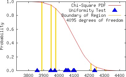
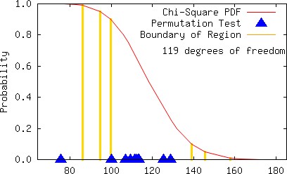
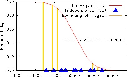
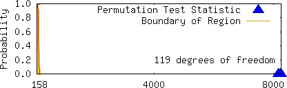
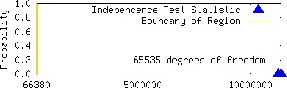
We next describe our method to filter out good multipliers. We conducted the following common tests by successively generating subsequences of length 6881280 ten times without reseeding for each multiplier found:
| Type of Test | Number of Tests | |
|---|---|---|
| Permutation | Four using k-tuples, k = 5,6,7,8 | |
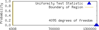
| Uniformity | One | |
| Independence | Six using k-dimensional hypercubes, k = 2,3,4,5,6,7 |
For each of the 110 tests, we assign a statistic σ using a χ2 goodness-of-fit test assuming the sample comes from a uniform distribution as follows:
| σ | Region of χ2 statistic | |
|---|---|---|
| 0 | 10% ≤ χ2 ≤ 90% | |
| 1 | 5% ≤ χ2 < 10% or 90% < χ 2 ≤ 95% | |
| 2 | 1% ≤ χ2 < 5% or 95% < χ2 ≤ 99% | |
| 3 | χ2 < 1% or χ2 > 99% |
What is the justification for this testing procedure? We normally expect to see the χ2 statistic to appear uniformly randomly distributed when the generated data appears uniformly randomly distributed. This means we also expect to see outliers occasionally. Ideally we would graph the results instead of computing the sum.
Example
Several multipliers were found using LLL reduction for the prime moduli 231 − 1 and 233 − 9 [27]. We list our results for all of these multipliers and a couple other multipliers which we found below for comparison purposes.
| Modulus | Multiplier | Period | LLL-spectral Result | ς |
|---|---|---|---|---|
| 231 − 1 | 598753959[27] | 2147483646 | 0.734350 | 43 |
| 231 − 1 | 117879879[27] | 2147483646 | 0.743094 | 36 |
| 231 − 1 | 629824009[27] | 2147483646 | 0.748798 | 47 |
| 231 − 1 | 1355089539[27] | 2147483646 | 0.749724 | 34 |
| 231 − 1 | 1101592370 | 2147483646 | 0.761410 | 17 |
| 233 − 9 | 8137022074[27] | 19739 | 0.753160 | 330 |
| 233 − 9 | 26891986 | 8589934582 | 0.756007 | 40 |
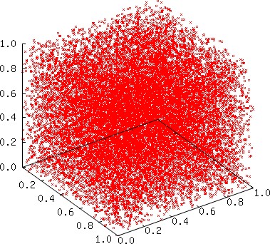
The multiplier 26891986 for the modulus 233 − 9 yields not only a full period but also a relatively small sum ς (40 << 330). We provide a few graphs below to visually show that the individual statistics are typically scattered when the multiplier is a good choice.
It is generally observed that poorly chosen constants for an LCG can be detected by a visual inspection of 2D or 3D graphs. Although the multiplier 8137022074 yields a 2D plot that does exhibit subtle patterns that might perhaps lead us to reject the multiplier, the 2D and 3D plots in this instance do not exhibit large gaps, which normally would be anticipated whenever the constants for the MCG are poorly chosen, i.e., the plots are unexpectedly good (because the empirical results are unsatisfactory), although such graphs are consistent with high LLL-spectral results. Below we plot 19739 points using the sequence
| s = { | 1 | (x0, x1, x2, …, x19738) }, |
m − 1 |
||
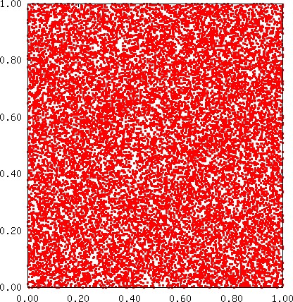
Surprisingly, for the vast majority of the multipliers found using LLL reduction for the modulus 233 − 9 , the statistic ς is relatively large. In other words, there are far fewer multipliers with a relatively small statistic in this case. We observe this phenomenon only for intermediate moduli (our tests are limited). For instance, for the prime modulus 238 − 45, only two of the 4096 multipliers found using LLL reduction may be considered satisfactory using our testing procedure! When the modulus is smaller, as in the case m = 231 − 1 , or larger than 249, we find far fewer large values of the statistic ς.
Interestingly, we found relatively more satisfactory multipliers (about 900 in each case) for moduli close to m = 233 for which m − 1 either has many factors or a relatively small factor besides two. Although we found over 8000 multipliers for both moduli m = 239 − 7 and m = 239 − 524281 with high LLL-spectral results, few passed our empirical tests and those that did pass our tests failed to provide a full period. For example, m = 239 − 7, the multiplier 407569451297 has an LLL-spectral result of 0.736035 and a low ς = 4, which are satisfactory but the period is only 7151242. For the modulus m = 239 − 524281, the multiplier 107627735285 has an LLL-spectral result of 0.676041 and a ς = 35 and the period is 13158220, which is relatively long (not a full period) compared to other multipliers that pass out tests. Thus the problem is not limited by the small quantity of satisfactory empirical results. Often the period is too short even when the LLL-spectral and empirical results are satisfactory. In the case of m = 249 − 81, we find many multipliers for which the LLL-spectral and empirical results are acceptable but for which the period is short (around 50+ million or less, which may be acceptable for some applications).
In review, we search for multipliers using our algorithm based on a fast implementation of LLL reduction. We then filter the multipliers by eliminating the ones that have either unacceptable empirical results based on a series of tests or too short period based on our modified version of Brent's algorithm. We provide a partial list of multipliers that pass our testing procedure for a few moduli in the table below. While these multipliers are good choices, our tests are not exhaustive and we could find better choices.
| 1327760490 | 2066353702 | 64673635 | 13496534 | 2115602258 |
| 1130487585 | 366987602 | 449666487 | 1179466207 | 1610952690 |
| 1144912594 | 750812715 | 237482926 | 589590877 | 63009789 |
| 1646375777 | 1982352019 | 276600333 | 1340326634 | 1172820338 |
| 849788117 | 1342204164 | 109002162 | 658081785 | 1332582004 |
| 214853381 | 89482149 | 602116046 | 593960624 | 1454735214 |
| 1306528138 | 62589812 | 1670073895 | 2126602119 | 396544957 |
| 359664239 | 1695987831 | 508747874 | 649683560 | 1355999881 |
| 1610666646 | 1438289155 | 2079645965 | 1136719287 | 611668365 |
| 1828435645 | 1878495191 | 1847615830 | 1237328482 | 1468948367 |
| 972970514 | 1010471390 | 126020853 | 706427382 | 1709121003 |
| 1101592370 | 1506604121 | 1512514978 | 824215950 | 1321742111 |
| 1888709996 | 995582175 | 1561995614 | 1304420267 | 1856996488 |
| 890285426 | 978341136 | 1151089329 | 2023442129 | 1385616379 |
| 1154363107 | 1700408166 | 942499575 | 1735119235 | 1443415006 |
| 968186004 | 857083457 | 1487296614 | 846315352 | 2084576224 |
| 389713771 | 614976766 | 1988625655 | 498035997 | 2091302020 |
| 884030647 | 563043968 | 1852865445 | 1605194785 | 1648446679 |
| 1259082738 | 1835824673 | 260994711 | 240447011 | 1147108816 |
| 15504300 | 1413287209 | 650491165 | 680854257 | 628062990 |
| 1435306322 | 927243288 | 1305700395 | 1434972591 | 593585162 |
| 1042208133 | 1894106185 | 1036034475 | 1673116415 | 241964875 |
| 434833139 | 843936096 | 1026031797 | 83283724 | 962428207 |
| 1766260325 | 522422173 | 153294169 | 544987095 | 885855294 |
| 1712991949 | 1186874058 | 1665120202 | 1481001151 | 1178284384 |
| 1300846825 | 100141984 | 1878222740 | 1194074653 | 1796829509 |
| 913776635 | 2047895118 | 584717610 | 1861041125 | 665538753 |
| 345309885 | 570635603 | 889304313 | 1370517560 | 1128124577 |
| 938844034 | 2062303428 | 1436861582 | 1786206933 | 1053597311 |
| 1580605747 | 1901854344 | 720358714 | 1236164771 | 2040072439 |
| 2227666520522988 | 2335245043818421572 | 2958048408930287532 | 2821497825880930668 |
| 6125433456171879 | 229869021091622116 | 541962160899652940 | 3645820036832622356 |
| 242991343497935 | 2986508760285856708 | 364313872487046284 | 2117980445355000731 |
| 385325382108333 | 1230401549344097348 | 4437343137438423668 | 1077327186057395324 |
| 0445622603323716 | 3404718480622991346 | 3632484698526789692 | 3040394404002739493 |
| 4716400480585236 | 4425050684624664868 | 601696678466323924 | 3360988063228378564 |
| 3245363233199204 | 305480126024544988 | 1140520979900998343 | 2904568835753732236 |
| 910487642975572 | 3573939289300556044 | 1437104732804195596 | 1111204688074489044 |
| 5423650086846141 | 3176158344253306828 | 3665506303834541868 | 529750891505220676 |
| 0272513680219020 | 757998535101219594 | 982506319620817612 | 510301227247225548 |
| 7476194856468218 | 1476746311225538452 | 2339344678753297700 | 2406547870037429612 |
| 308330264249580 | 2028107709143540196 | 460465672511139916 | 2169322410029413884 |
| 6234903618635836 | 2836325001576828756 | 3304850999237510764 | 1302692003016593727 |
| 9507500607942393 | 1127184225209561420 | 2442328367503098604 | 3525967833252807900 |
| 3517735631097212 | 254533705499448356 | 3216739265730783020 | 2734845951024098108 |
| 9762161018925836 | 3143250031667232428 | 4312569826513122964 | 2858990330270135956 |
| 818812215302820 | 3505111250052047420 | 142682684051643767 | 2924706175868748540 |
| 9091477482083836 | 3005708043498447004 | 1122404151658602356 | 2384376175079003364 |
| 2101648724486855 | 3049914937445631084 | 2485606123337880225 | 3737901350162908743 |
| 3087629853475092 | 2820800426820749716 | 1803501089697376940 | 1322520419430537292 |
| 6375748891921916 | 771883998081009342 | 1514926988797966303 | 2213119349169260508 |
| 031080726473732 | 2243945721847679725 | 2930516100542645740 | 4494970451474388404 |
| 7462914720430958 | 3843182323716420380 | 2876990204610411756 | 1007531718334738490 |
| 8538904338130612 | 2606475706061829691 | 960695606911668116 | 2782767896275353612 |
| 7053581384735532 | 1643282104386383980 | 670108774451549844 | 1001393204888569492 |
| 8585308547598203 | 2418232767452531692 | 1621277272908803724 | 4008104371906474908 |
| 7809888395679756 | 1049643446522008484 | 432127321738792164 | 1789457316119133228 |
| 312008784666244 | 1849084705355803389 | 4261613820926935399 | 857519200068935628 |
| 0472151709439338 | 4067814427609890436 | 1273491878580529124 | 2083357865738529211 |
| 8098840758717236 | 3898454276482771700 | 2383006420636971996 | 447971768444903140 |
| 8097943894898732 | 2442060819726853316 | 1533254051312395243 | 468986501493944828 |
| 249454169311180 | 1188318551523486772 | 2593239100320542884 | 1683383931902134724 |
| 5048131329874245129129 | 6970857753449530850 | 6420278701347409430 | 5124525484560574678 |
| 3599012081437622174 | 9033130285246985478 | 3135883546616849630 | 5450100294142127183 |
| 5230828488753169785 | 5277564623835390478 | 1243915603764351534 | 3067675794346700338 |
| 1164142900299891771 | 1690244713649970294 | 8504294721320585030 | 1982429857622105466 |
| 5863122408574880490 | 7488297927170703726 | 1192417868866640021 | 4674946439731140607 |
| 2161553242107985838 | 3693270853121744274 | 2723638313981663842 | 2583372058471374662 |
| 5583226340227159521 | 7440483159998091718 | 6865597922945174018 | 6710640246843790433 |
| 8130017674206960802 | 1355888514815117818 | 66935293183612951 | 7310597557252160706 |
| 2193035004633415366 | 698553738790551194 | 5359281404268310005 | 8724299514156051935 |
| 126418711700522650 | 3558263172428606031 | 6343443902471568174 | 4485294600469307766 |
| 7041410690023337563 | 7578608487980007799 | 253175814488353254 | 2347700846709651015 |
| 2138588662245218566 | 8408227919743527230 | 5206346059077753018 | 1955988046358844486 |
| 8189359621998424622 | 3616566817062986114 | 6424355341835960642 | 2500937059175260802 |
| 8080320067683804887 | 8033051016217168982 | 7321992163586838902 | 6411023698701546182 |
| 1769007136379980686 | 7783932335745702394 | 5558975998246609070 | 2143403440715322422 |
| 3179570434846579489 | 4945674464234686695 | 4695325265498138958 | 5288198982489587626 |
| 7762145188453129894 | 6245073051208444365 | 1478438406335434706 | 2309620102346487126 |
| 2287775950289931630 | 2457532858703768094 | 6610727231368630747 | 905762158313624865 |
| 870491490180669699 | 9197167186577252565 | 3870451705883074774 | 439605922369016570 |
| 4359681192108683725 | 643024978184937358 | 8162972527107683162 | 4667597220755320922 |
| 1937140893319420210 | 5487491960955870086 | 6672346787909502191 | 719372909398164950 |
| 3760870210522814318 | 1827366899773106907 | 8652243963382490303 | 5176898528264328250 |
| 1773166088840501934 | 2479698328010538454 | 9087242916220307793 | 2289446703802487557 |
| 400065671079016742 | 1035122893537674026 | 6561247231059429639 | 9169751783082340538 |
| 6564255993928279035 | 3997015511275500730 | 549512076501724846 | 1925625704083580246 |
| 844694661116743062 | 1456029575323840666 | 7410714248380123986 | 8688101763314670602 |
| 5595565586107992950 | 5611696577798111118 | 3927998942213401347 | 1561798619548458430 |
| 598858993587313666 | 8205566993320371494 | 7154943775958131514 | 5670532371588444962 |
| 9054079806224684046 | 7044308632905183510 | 7855708569000872254 | 4546508663771071157 |
| 2048336232069601622 | 192296947391005798 | 6940449059354001403 | 4595997938451814114 |
| 4832871382696361267 | 123352434606157734 | 676201409278475890 | 4217132583335612998 |
| 9077402637247533766 | 9035191738883420082 | 2228114199495086142 | 7909033251671519 |
For each experiment, we develop both MPI and hybrid MPI + OpenMP code. For the MPI version, we use 128 MPI processes on 32 nodes. For the hybrid version, we use 32 MPI processes on 32 nodes with 4 threads per node, which yields a total of 128 threads.
For all tests, we employ the same prime modulus m = 8589934583 = 233 − 9, and the same initial seed x0 = 7927, which is a primitive root of m. We chose this modulus because we were able to find ample multipliers with full period. Although our choice of a seed is arbitrary and some authors suggest picking a seed randomly, we would recommend choosing one randomly from a set of tested seeds because the period can be affected by the choice of seed for large moduli. Using an assigned seed and multiplier, each process or thread generates pseudorandom numbers in parallel as needed using Algorithm 2.
Each experiment consists of two parts. In the first part, each process or thread uses the same multiplier, namely 1178748639 (listed first in table below), and a different seed. We assign a seed to each process or thread uniquely according to its MPI rank and OpenMP thread number using a single MCG for all processes/threads
| 1178748639 | 1504451367 | 1438843832 | 1508982646 |
| 2039663820 | 1498584416 | 1753099100 | 1264049400 |
| 420951726 | 944773179 | 1894605422 | 1972037996 |
| 2145391955 | 1290515899 | 821331287 | 233089823 |
| 815719265 | 1037449050 | 391368831 | 1619611282 |
| 174343685 | 36512342 | 83440728 | 469601921 |
| 1887658788 | 409426010 | 710163604 | 720184858 |
| 642944870 | 165253310 | 2030930240 | 1015182040 |
| 1399937605 | 964731408 | 1370458820 | 928764526 |
| 835644228 | 964138849 | 771690904 | 2100758807 |
| 2058614442 | 1736063227 | 388665714 | 783217427 |
| 1981572859 | 297867486 | 1441424772 | 1649895453 |
| 1959842942 | 1855047552 | 1105029878 | 207427210 |
| 967163134 | 2073682087 | 159098215 | 1721887127 |
| 504646265 | 1483353159 | 1485525714 | 1538189469 |
| 1716278914 | 2033983412 | 2078532603 | 1926327885 |
| 1959643358 | 154598950 | 406575269 | 36921595 |
| 839205172 | 1494766337 | 1210100711 | 1837727164 |
| 1789532978 | 274166327 | 685199652 | 1183031368 |
| 2109888739 | 347221270 | 436678419 | 380986609 |
| 1171151118 | 1389829650 | 1912037874 | 324737772 |
| 1636694774 | 1508450362 | 1755102432 | 1619085308 |
| 617918706 | 1989869210 | 984783477 | 259413370 |
| 1316480107 | 1837397190 | 1240911029 | 197185544 |
| 830682663 | 1977680361 | 1403997604 | 291188364 |
| 1428272847 | 160535591 | 1093106588 | 1971097235 |
| 1899338587 | 574974465 | 707574314 | 743571448 |
| 787295652 | 2055016389 | 1786492583 | 447846030 |
| 614468563 | 198700516 | 627010989 | 1587207860 |
| 249082425 | 1132873853 | 717740897 | 901967693 |
| 1167409652 | 1363068688 | 1627762155 | 581967324 |
| 705969097 | 709166350 | 1570040924 | 429303093 |
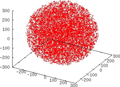
| C | ≈ | (4 ⁄ 3) π (300)3 | = | π | . |
232 |
6003 |
6 |
| Test | Approximation to π MPI/Hybrid |
|---|---|
| same multiplier, different seed | 3.1415769774466753 |
| different multiplier, same seed | 3.1415196494199336 |
Although we do not expect to see a difference between MPI and hybrid (except in terms of timing since even though the sum is computed differently, it is an integral sum), we would have expected greater accuracy when using different multipliers, which is not observed in this experiment. On the other hand, we do not lose a single digit of accuracy by using the same seed with different multipliers. To further check the quality of the distributions produced, we ran another test using MPI with different multipliers in which each MPI process generates a much smaller number of points, specifically 128 points per process, and collected all of the points that coincide with the sphere from all processes. The resulting graph displayed below indicates a satisfactory distribution.
| 128! = | 385620482362580421735677065923463640617493109590223590278828403276373402 |
| 575165543560686168588507361534030051833058916347592172932262498857766114 | |
| 955245039357760034644709279247692495585280000000000000000000000000000000 |
There is a simple and fast way to generate a “pseudorandom permutation.” Choose any arbitrary permutation initially. Successively generate the next permutation using the previous permutation as follows. Uniformly randomly pick any position and swap the element in this position with the last element. After each swap the element in the rightmost position is in its final position. Recursively, uniformly randomly pick a position corresponding to the elements excluding those elements in the tail that have already been placed and swap with the last element excluding the tail. Hence it takes only n − 1 swaps (and pseudorandom number generations) to generate the next permutation of a list with n elements. This method is amazing because it is not only fast but also produces permutations as if sampling from a uniform distribution [36]. In our tests, we found the generation of pseudorandom permutations (as described) seems to come from a uniform distribution even when the MCG used to swap elements fails many tests.
Our main interest is to generate permutations in parallel. Obviously two distinct processes should not generate the same permutation. Yet it is not enough to simply avoid the generation of the same permutations from among the incredibly vast number of them. Collectively, the permutations should appear as if they come from a uniform distribution. Ideally, this sampling is done independently without communication for the sake of speed.
In our experiment, each process (or thread) uses the same algorithm and an MCG as previously described to swap elements. Each process generates 20484 permutations of a list with 128 elements, starting with the same initial permutation which is arbitrarily chosen to be
We do not store and collect the actual permutations. Instead we store a single number to represent each permutation. There is a natural number to associate with each permutation. List all permutations in increasing lexicographical order and associate the position of each permutation in the ordered list with that permutation, e.g., {0,1,…,127} is assigned the number 0 and {127,126,…,0} the familiar number 128!. The only flaw with this numbering scheme is the numbers are unwieldy. Although sorting is really out of the question, figuring out the position is fast (much like looking up a phone number - if the first digit is k then we know the permutation comes after all permutations whose first digit is j with j < k, etc.). A solution to deal with the unwieldy numbers is to apply the same nice operation which is used to generate pseudorandom numbers themselves, i.e., modulo operation. Thus, after we generate a permutation we calculate its ‘number’ by computing its position using modular arithmetic, which is relatively costly in terms of operations compared to generating the permutation itself! We choose a reasonably large modulus M and precompute factorial(k) = k! mod M for k ∈ {1,…,n−1}, where n is the length of the list. We present our algorithm to compute the numbers assigned to a permutation next.
Algorithm 7: Map Permutation to an Integer ζ
In our experiment we use the modulus M = 232 in the preceding algorithm because we easily obtain suitable data for the diehard tests. We collect all numbers computed for every permutation by all processes (threads) and print the numbers to a file. The resulting files were exactly the same for the MPI and hybrid versions. We then ran diehard tests on these files. Nearly all of the diehard tests are clearly passed whether we use the same multiplier and different seeds or different multipliers and the same seed. Only a couple of the diehard tests are not clearly passed but the same failures occur regardless of the experiment (both parts). Although it is sufficient to use different seeds in this case, the results are also satisfactory using different multipliers.
We have significantly improved the performance of an LLL reduction implementation and presented an algorithm to find many candidate multipliers for a prime modulus. We have shown that some multipliers with high LLL-spectral results (including some which are published [27]) are unsatisfactory. We also discovered an unexpected phenomenon for certain intermediate moduli: the vast majority of the multipliers with high LLL-spectral results are unsatisfactory based on empirical tests. We introduced a fast empirical testing procedure to select good multipliers from thousands of multipliers with satisfactory LLL-spectral results. We also introduced a modification of Brent's algorithm to quickly discover short periods, which we have shown is useful because the period is frequently short even when the LLL-spectral and empirical results are acceptable. We also introduced an algorithm to assign numbers to a permutation for statistical analysis.
It is not convincing to draw conclusions on the basis of a small number of experiments. More experiments are needed. Regardless, the only way to know whether a method of parallel number generation is adequate for an application is to conduct tests to assess the quality for each implementation. Scalability is a concern especially when using different seeds. We advocate using different multipliers chosen as described herein. Our experiments produced satisfactory results using different multipliers. For different runs we recommend using a different seed but rather than choosing a seed completely randomly, we recommend uniformly randomly picking a seed from a set that has been tested in advance.
For some moduli (not all such as 239 − 7) we found plenty of multipliers with both high LLL-spectral results and low ς statistics. It is unclear how to select multipliers from a large set of multipliers that will work best in parallel. It is impractical to exhaustively test all possible subsets with k elements (scaling to k processors) from a set of N multipliers (unless k ≈ N), e.g., the number of subsets having 128 multipliers from a set of 1024 multipliers has 167 digits.